Multi-armed Bandits

Tabular Solution Methods

Now we consider the simplest forms: the state and action spaces are small enough for the approximate value functions to be represented as arrays, or tables.

Multi-armed Bandits

Special case: only a single state, simplified setting that does not involve learning to act in more than one situation (nonassociative setting)

A k-armed Bandit Problem

Each of the k actions has an expected or mean reward given that that action is selected (value of that action)

$A_t$ - action selected on time step $t$

$R_t$ - corresponding reward

$q_*(a)$ - value of an arbitrary action $a$

\[q_*(a) \dot{=} \mathbb{E}[R_t \vert A_t=a]\]

$Q_t(a)$ - estimated value of $a$ at $t$

• Greedy actions: at any time step there is at least one action whose estimated value is greatest
  • Exploiting: select one of the greedy actions
  • Exploring: select one of the nongreedy actions

Exploitation is the right thing to do to maximize the expected reward on the one step, but exploration may produce the greater total reward in the long run. The need to balance exploration and exploitation is a distinctive challenge in RL.

Action-value Methods

Methods for estimating the values of actions and for using the estimated to make action selection decisions.

One natural way to estimate: average the rewards actually received (Sample-average method)

\[Q_t(a) \dot{=} \frac{\mathrm{sum~of~rewards~when}~a~\mathrm{taken~prior~to~}t}{\mathrm{number~of~times~}a~\mathrm{taken~prior~to~}t} = \frac{\sum_{i=1}^{t-1} {R_{i} \cdot {\mathbb{1}_{A_i=a}} }} {\sum_{i=1}^{t-1} {\mathbb{1}_{A_i=a}}}\]

Simplest action selection rule: select one of the actions with the highest estimated value (one of the greedy actions)

\[A_t \dot{=} \mathrm{argmax}_a Q_t(a)\]

A simple alternative: with small probability $\varepsilon$, select randomly from among all the actions with equal probability, independently of the action-value estimates ($\varepsilon$-greedy methods)

Incremental Implementation

Compute sample averages in a computationally efficient manner, with constant memory and constant per-time-step computation

$R_i$ - reward received after the $i$th selection of this action

$Q_n$ - estimate of this action’s value after it has been selected $n-1$ times

\[Q_n \dot{=} \frac{R_1+R_2+\cdots+R_{n-1}}{n-1}\]

However, each additional reward would require additional memory and computation

Devise incremental formulas:

\[\begin{align} Q_{n+1} &= \frac{1}{n}\sum_{i=1}^n {R_i}\\ &= \frac{1}{n}\Big(R_n + \sum_{i=1}^{n-1} {R_i}\Big)\\ &= \frac{1}{n}\Big(R_n + (n-1)Q_n\Big)\\ &= Q_n + \frac{1}{n}[R_n-Q_n]\\ \end{align}\]

The formulas hold even for $n=1$, obtaining $Q_2=R_1$ for arbitrary $Q_1$

General form:

\[NewEstimate \leftarrow OldEstimate + StepSize[Target-OldEstimate]\]

• $[Target-OldEstimate]$ is an error in the estimate

• Denote step-size parameter by $\alpha$ or $\alpha_t(a)$

Pseudocode for a complete bandit algorithm using incrementally computed sample averages and $\varepsilon$-greedy action selection:

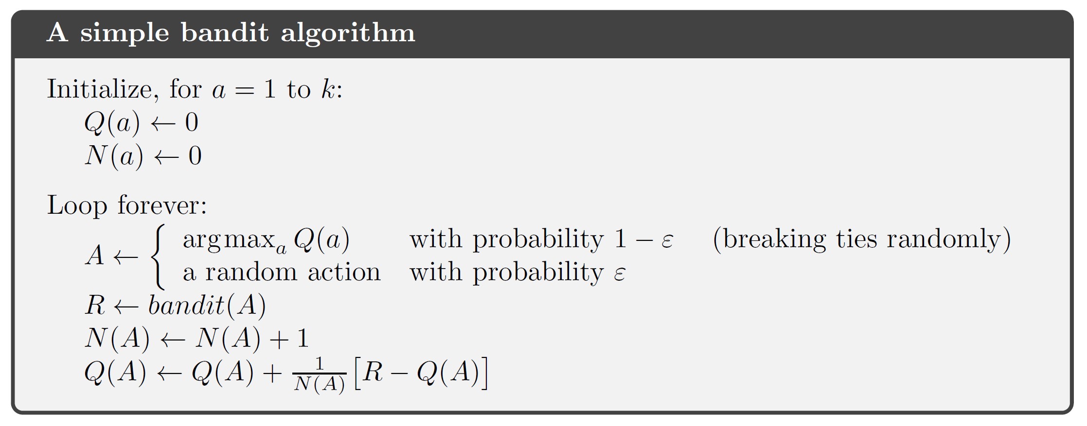A simple bandit algorithm

The averaging methods above are appropriate for stationary bandit problems (the reward probabilities do not change over time)

Tracking a Nonstationary Problem

For nonstationary problems, give more weight to recent rewards than to long-past rewards. One of the most popular ways is to use a constant step-size parameter.

Modify the incremental update rule for $Q_n$:

\[Q_{n+1} \dot{=} Q_n + \alpha [R_n-Q_n]\]

where $\alpha\in (0,1]$ is constant.

$Q_{n+1}$ is a weighted average of past rewards and the initial estimate $Q_1$:

\[\begin{align} Q_{n+1} &= Q_n+\alpha[R_n-Q_n]\\ &= \alpha R_n + (1-\alpha)Q_n\\ &= \alpha R_n + (1-\alpha)[\alpha R_{n-1} + (1-\alpha)Q_{n-1}]\\ &= \alpha R_n + (1-\alpha)\alpha R_{n-1} + (1-\alpha)^2 Q_{n-1}\\ &= \cdots\\ &= (1-\alpha)^n Q_1 + \sum_{i=1}^n {\alpha(1-\alpha)^{n-i} R_i}\\ \end{align}\]

Sometimes it’s convenient to vary the step-size parameter from step to step, like the choice $\alpha_n(a)=\frac{1}{n}$ in the sample-average method. But convergence is not guaranteed for all choices of ${\alpha_n(a)}$. Conditions required to assure convergence with probability 1:

\[\sum_{n=1}^\infty \alpha_n(a)=\infty \quad \mathrm{and} \quad \sum_{n=1}^\infty \alpha_n^2(a)<\infty\]

For the sample-average case, both conditions are met, but for the case of constant step-size parameter, the second case is not met, indicating the estimates never completely converge but continue to vary in response to the most recently received rewards. This is desirable in a nonstationary environment.

Optimistic Initial Values

• Methods dependent on the initial action-value estimates $Q_1(a)$ are biased by their initial estimates.

• Initial action values can be used as a simple way to encourage exploration.

Exploration is needed because there is always uncertainty about the accuracy of the action-value estimates

• Any method that focuses on the initial conditions is unlikely to help with the general nonstationary case.

Upper-Confidence-Bound (UCB) Action Selection

Select among the non-greedy actions according to their potential for actually being optimal, taking into account both how close their estimates are to being maximal and the uncertainties in those estimates

$\varepsilon$-greedy action selection forces the non-greedy actions to be tried indiscriminately, with no preference for those that are nearly greedy or particularly uncertain.

One effective way: select actions according to

\[A_t \dot{=} \mathrm{argmax}_a \left[ Q_t(a) + c\sqrt{\frac{\ln t}{N_t(a)}} ~\right]\]

where:

• $N_t(a)$ - the number of times that action $a$ has been selected prior to time $t$
• $c>0$ controls the degree of exploration

The idea of this upper confidence bound (UCB) action selection is that the square-root term is a measure of the uncertainty or variance is the estimate of $a$’s value. The quantity being max’ed over is thus a sort of upper bound on the possible true value of action $a$, with c determining the confidence level.

Gradient Bandit Algorithms

Consider learning a numerical preference for each action $a$, $H_t(a)\in\mathbb{R}$

The preference has no interpretation in terms of reward. Only the relative preference is important.

Action probabilities are determined according to a soft-max distribution:

\[\mathrm{Pr}\{A_t=a\} \dot{=} \frac{e^{H_t(a)}}{\sum_{b=1}^k {e^{H_t(b)}}} \dot{=} \pi_t(a)\]

$\pi_t(a)$ - probability of taking action $a$ at time $t$

A natural learning algorithm for soft-max distribution action preferences based on the idea of stochastic gradient ascent:

On each step, after selecting action $A_t$ and receiving the reward $R_t$,update the action preferences:

\[\begin{align} H_{t+1}(A_t) & \dot{=} H_t(A_t) + \alpha(R_t-\bar{R_t})(1-\pi_t(A_t)), & \mathrm{and}\\ H_{t+1}(a) & \dot{=} H_t(a)-\alpha(R_t-\bar{R_t})\pi_t(A_t), & \forall a \neq A_t\\ \end{align}\]

where:

• $\alpha>0$ - step-size parameter
• $\bar{R_t}\in\mathbb{R}$ - average of the rewards up to but not including time $t$ ($\bar{R_1}\dot{=}R_1$)

Associative Search (Contextual Bandits)

Extend nonassociative tasks to the associative setting

Nonassociative tasks do not need to associate different actions with different situations.

An associative search task (often now called contextual bandits) involves both trial-and-error learning to search for the best actions, and association of these actions with the situations in which they are best.

Associative search tasks are intermediate between the k-armed bandit problem and the full RL problem. They involve learning a policy, but each action affects only the immediate reward. If actions are allowed to affect the next situation as well as the reward, then we have the full RL problem.

Summary

• Several simple ways of balancing exploration and exploitation
  • $\varepsilon$-greedy methods choose randomly a small fraction of the time
  • UCB methods choose deterministically but achieve exploration by subtly favoring at each step the actions that have so for received fewer samples
  • Gradient bandit algorithms estimate not action values, but action preferences, and favor the more preferred actions in a graded, probabilistic manner using a soft-max distribution
• To compare which methods is best, produce learning curves for algorithms and parameter settings

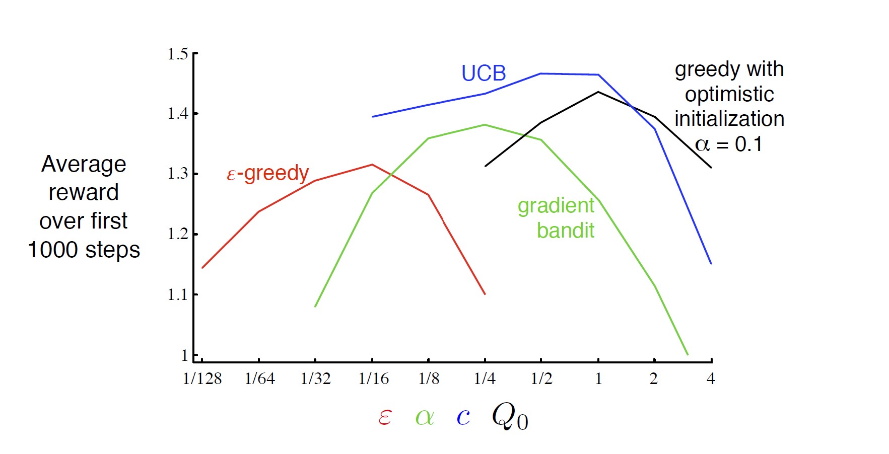A parameter study of the various bandit algorithms on the 10-armed testbed