
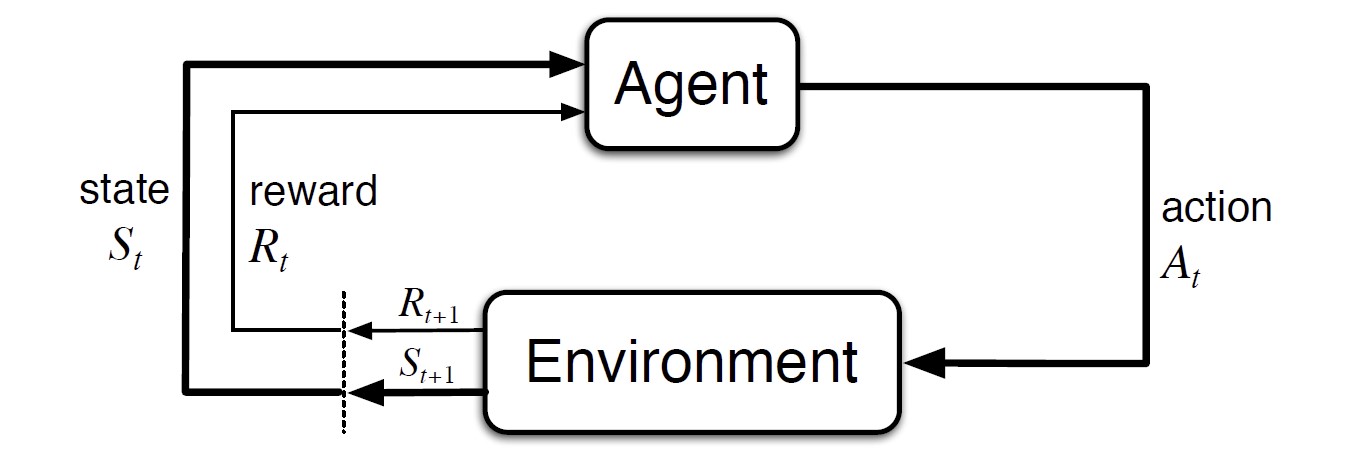
The Agent-Environment Interface
- Agent: learner and decision maker
- Environment: everything outside the agent
 The agent-environment interaction in a MDP
Interaction at discrete time steps: $t=0,1,2,3,\dots$
- At each time step $t$, the agent receives the environment’s state, $S_t\in\mathcal{S}$, and on that basis selects an action $A_t\in\mathcal{A(s)}$
- One time step later, the agent receives a numerical reward, $R_{t+1} \in\mathcal{R}\subset\mathbb{R}$ as a consequence of its action, and finds itself in a new state, $S_{t+1}$
MDP and Agent $\rightarrow$ a sequence or trajectory: $S_0,A_0,R_1,S_1,A_1,R_2,S_2,A_2,R_3,\dots$
- In a finite MDP, the sets of states, actions and rewards ($\mathcal{S}$, $\mathcal{A}$, $\mathcal{R}$) all have a finite number of elements.
- $R_t$ and $S_t$ have well defined discrete probability distributions dependent only on the preceding state and action
- Dynamics of MDP
- $p$ completely characterize the environment’s dynamics
- Markov property: the state must include information about all aspects of the past agent-environment interaction that make a difference for the future
From $p$ we can compute the anything about the environment, such as:
\[p(s'\vert s,a)=\sum_{r\in\mathcal{R}} {p(s',r\vert s,a)}\]
- state-transition probabilities:
\[r(s,a) = \sum_{r\in\mathcal{R}}r\sum_{s'\in\mathcal{S}}p(s',r\vert s,a)\]
- expected rewards for state-action pairs:
\[r(s,a,s')=\sum_{r\in\mathcal{R}}\frac{p(s',r\vert s,a)}{p(s'\vert s,a)}\]
- expected rewards for state-action-next-state triples:
MDP Framework is a considerable abstraction and can be applied to many different problems in many different ways.
Example: Pick-and-Place Robot
Consider using reinforcement learning to control the motion of a robot arm in a repetitive pick-and-place task. If we want to learn movements that are fast and smooth, the learning agent will have to control the motors directly and have low-latency information about the current positions and velocities of the mechanical linkages. The actions in this case might be the voltages applied to each motor at each joint, and the states might be the latest readings of joint angles and velocities. The reward might be +1 for each object successfully picked up and placed. To encourage smooth movements, on each time step a small, negative reward could be given as a function of the moment-to-moment jerkiness of the motion.
Goals and Rewards
Reward Hypothesis:
That all of what we mean by goals and purposes can be well thought of as the maximization of the expected value of the cumulative sum of a received scalar signal called reward.
It is critical that the rewards we set up truly indicate what we want accomplished. The reward signal is not the place to impart to the agent prior knowledge about how to achieve what we want it to do. The reward signal is the way of communicating to the agent what we want achieved, not how we want it achieved.
Returns and Episodes
The agent’s goal is to maximize the cumulative reward in the long run, called the expected return $G_t$
Simplest case: sum of rewards
\[G_t \dot{=} R_{t+1}+R_{t+2}+\cdots+R_T\]where $T$ is a final time step.
Episodic Tasks
There is a natural notion of final time step, when the agent-environment interaction breaks naturally into subsequences called episodes. Each episode ends in a special state called the terminal state. Tasks with episodes are called episodic tasks.
In episodic tasks, sometimes distinguish the set of all nonterminal states $\mathcal{S}$, from the set of all states plus the terminal state $\mathcal{S}^+$.
Continuing Tasks
Continuing tasks: the agent-environment interaction does not break naturally into identifiable episodes, but goes no continually without limit ($T=\infty$)
Introduce discounting: the agent chooses $A_t$ to maximize the expected discounted return
\[G_t \dot{=} R_{t+1} + \gamma R_{t+2} + \gamma^2R_{t+3} +\cdots = \sum_{k=1}^\infty {\gamma^k R_{t+k+1}}\]where $\gamma\in[0,1]$ is called the discount rate. As $\gamma$ approaches 1, the return objective takes future rewards into account more strongly; the agent becomes more farsighted.
Returns at successive time steps are related to each other (Define $G_T=0$):
\[\begin{align} G_t \dot{=}& R_{t+1} + \gamma R_{t+2} + \gamma^2R_{t+3} +\gamma^3 R_{t+4}\cdots\\ =& R_{t+1} + \gamma(R_{t+2}+\gamma R_{t+3}+\gamma^2R_{t+4})\\ =& R_{t+1} + \gamma G_{t+1}\qquad \forall t<T \\ \end{align}\]Unified Notation for Episodic and Continuing Tasks
$S_{t,i}$ - State representation at time $t$ of episode $i$
$A_{t,i},~\pi_{t,i},~T_i$
Always consider a particular episode, write $S_t$ to refer to $S_{t,i}$
Unify the definition of return: consider episode termination to be the entering of a special absorbing state that transitions only to itself and generates only rewards of 0
Define the return:
\[G_t \dot{=} \sum_{k=t+1}^T {\gamma^{k-t-1} R_k}\]Policies and Value Functions
Value functions are functions of states (or of state-action pairs) that estimate how good it is for the agent to be in a given state (or how good it is to perform a given action in a given state).
A policy is a mapping from states to probabilities of selecting each possible action. RL specify how the agent’s policy is changed as a result of its experience.
$v_\pi(s)$ - value function of a state $s$ under a policy $\pi$ (state-value function for policy $\pi$)
For MDP, define $v_\pi$ by
\[v_\pi(s) \dot{=} \mathbb{E}_\pi[G_t\vert S_t=s] = \mathbb{E}_\pi\left[ \sum_{k=0}^\infty {\gamma^k R_{t+k+1}\Big\vert S_t=s} \right]\quad \forall s\in\mathcal{S}\]$q_\pi(s,a)$ - value function of taking action $a$ in state $s$ under a policy $\pi$ (action-value function for policy $\pi$)
\[q_\pi(s) \dot{=} \mathbb{E}_\pi[G_t\vert S_t=s, A_t=a]= \mathbb{E}_\pi\left[ \sum_{k=0}^\infty {\gamma^k R_{t+k+1}\Big\vert S_t=s, A_t=a} \right]\]The value functions $v_\pi$ and $q_\pi$ can be estimated from experience by averaging over many random samples of actual returns (Monte Carlo methods).
Bellman equation for $v_\pi$ (recursive relationships similar to return):
\[\begin{align} v_\pi(s) \dot{=}& \mathbb{E}_\pi[G_t\vert S_t=s] \\ =& \mathbb{E}_\pi[R_{t+1}+\gamma G_{t+1}\vert S_t=s]\\ =& \sum_a {\pi(a\vert s)}\sum_{s'}\sum_r p(s',r\vert s,a)\Big[r+\gamma\mathbb{E}_\pi[G_{t+1}\vert S_{t+1}=s']\Big]\\ =& \sum_a {\pi(a\vert s)}\sum_{s',r}p(s',r\vert s,a)\Big[r+\gamma v_\pi(s')\Big]\\ \end{align}\]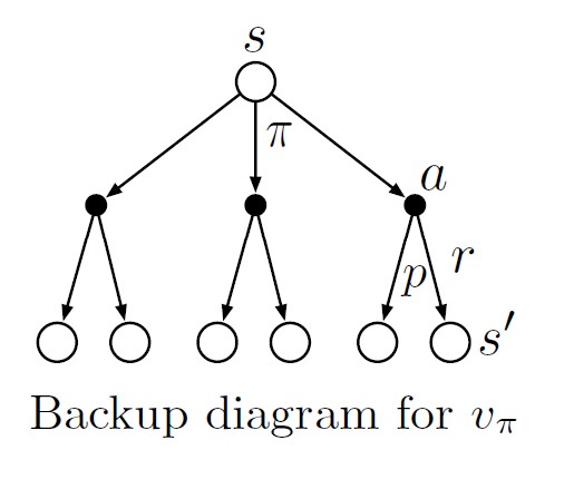
Bellman equation expresses a relationship between the value of a state and the values of its successor states. Backup diagrams show relationships that form the basis of the update or backup operations. These operations transfer value information back to a state (or a state-action pair) from its successor states (or state-action pairs)
Optimal Policies and Optimal Value Functions
Define a policy $\pi$ is better than or equal to $\pi’$ ($\pi\geq\pi’$) if and only if $v_\pi(s)\geq v_{\pi’}(s),\forall s\in\mathcal{S}$
Optimal policies $\pi_\ast$ (may be more than one) share the same state-value function and action-value function
Define optimal state-value function $v_\ast$ and optimal action-value function $q_\ast$:
\[\begin{align} v_*(s) &\dot{=} \max_\pi v_\pi(s) \qquad \forall s\in\mathcal{S}\\ q_*(s) &\dot{=} \max_\pi q_\pi(s,a) \quad \forall s\in\mathcal{S}, a\in\mathcal{A}(s)\\ \end{align}\]Write $q_\ast$ in terms of $v_\ast$
\[q_*(s,a)=\mathbb{E} [R_{t+1}+\gamma v_*(S_{t+1})\vert S_t=s,A_t=a]\]Bellman Optimality Equation
\[\begin{align} v_*(s) &= \max_{a\in\mathcal{A}(s)} q_{\pi_*}(s,a)\\ &= \max_a \mathbb{E}_{\pi_*}[G_t\vert S_t=s,A_t=a]\\ &= \max_a \mathbb{E}_{\pi_*}[R_{t+1}+\gamma G_{t+1} \vert S_t=s,A_t=a]\\ &= \max_a \mathbb{E}_{\pi_*}[R_{t+1}+\gamma v_*(S_{t+1})\vert S_t=s,A_t=a]\\ &= \max_a \sum_{s',r} p(s',r\vert s,a)[r+\gamma v_*(s')]\\ \end{align}\] \[\begin{align} q_*(s,a) &= \mathbb{E}\Big[R_{t+1}+\gamma \max_{a'}q_*(S_{t+1},a')\Big\vert S_t=s,A_t=a\Big]\\ &= \sum_{s',r} p(s',r\vert s,a) \big[r+\gamma \max_{a'}q_*(s',a')\big]\\ \end{align}\]If we have the optimal value function $v_\ast$, then the actions that appear best after a one-step search will be optimal actions.
The one-step greedy policy is actually optimal in the long-term sense because $v_\ast$ already takes into account the reward consequences of all possible future behavior. By means of $v_\ast$, the optimal expected long-term return is turned into a quantity that is locally and immediately available for each state.
With $q_\ast$, the agent does not even have to do a one-step-ahead search: for any state $s$, it can simply find any action that maximizes $q_\ast(s,a)$
Explicitly solving the Bellman optimality equation provides one route to finding an optimal policy, and thus to solving the RL problem. However, this solution is rarely directly useful.
Optimality and Approximation
Optimality is an ideal. Framing of RL problem forces us to settle for approximations.
The online nature of RL makes it possible to approximate optimal policies in ways that put more effort into learning to make good decisions for frequently encountered states, at the expense of less effort for infrequently encountered states.
Comments powered by Disqus.