
DP can be used to compute optimal policies given a perfect model of the environment as a MDP.
Key idea: use value functions to organize and structure the search for good policies
Review: Bellman optimality equations
\[\begin{align} v_\ast(s) &= \max_a \mathbb{E}_{\pi_\ast}[R_{t+1}+\gamma v_\ast(S_{t+1})\vert S_t=s,A_t=a]\\ &= \max_a \sum_{s',r} p(s',r\vert s,a)[r+\gamma v_\ast(s')]\\ \end{align}\] \[\begin{align} q_\ast(s,a) &= \mathbb{E}\Big[R_{t+1}+\gamma \max_{a'}q_\ast(S_{t+1},a')\Big\vert S_t=s,A_t=a\Big]\\ &= \sum_{s',r} p(s',r\vert s,a) \big[r+\gamma \max_{a'}q_\ast(s',a')\big]\\ \end{align}\]
Policy Evaluation (Prediction)
Policy evaluation: compute the state-value function $v_\pi$ for an arbitrary policy $\pi$
Recall:
\[\begin{align} v_\pi(s) \dot{=}& \mathbb{E}_\pi[G_t\vert S_t=s] \\ =& \mathbb{E}_\pi[R_{t+1}+\gamma G_{t+1}\vert S_t=s]\\ =& \sum_a {\pi(a\vert s)}\sum_{s'}\sum_r p(s',r\vert s,a)\Big[r+\gamma\mathbb{E}_\pi[G_{t+1}\vert S_{t+1}=s']\Big]\\ =& \sum_a {\pi(a\vert s)}\sum_{s',r}p(s',r\vert s,a)\Big[r+\gamma v_\pi(s')\Big]\\ \end{align}\]where $\pi(a\vert s)$ - probability of taking action $a$ in state $s$ under policy $\pi$
If the environment’s dynamics are completely known, the equation is system of $\vert\mathcal{S}\vert$ simultaneous linear equations in $\vert\mathcal{S}\vert$ unknowns ($v_\pi(s),s\in\mathcal{S}$)
Iterative Policy Evaluation
Consider a sequence of approximate value functions $v_0,v_1,v_2,\dots$
- $v_0$ is chose arbitrarily (except that the terminal state must be given value 0)
- Each successive approximation is obtained by using Bellman equation for $v_\pi$ as an update rule:
- ${v_k}$ converge to $v_\pi$ as $k\rightarrow\infty$
- Expected Update: each iteration updates the value of every state once to produce new approximate value function $v_{k+1}$
In-place algorithm
To write a computer program to implement iterative policy evaluation, we have to use two arrays, one for the old values $v_k(s)$, and one for the new values $v_{k+1}(s)$.
Alternatively, we could use one array and update the values “in place” (each new value immediately overwrites the old one). The in-place algorithm converges to $v_\pi$ faster.
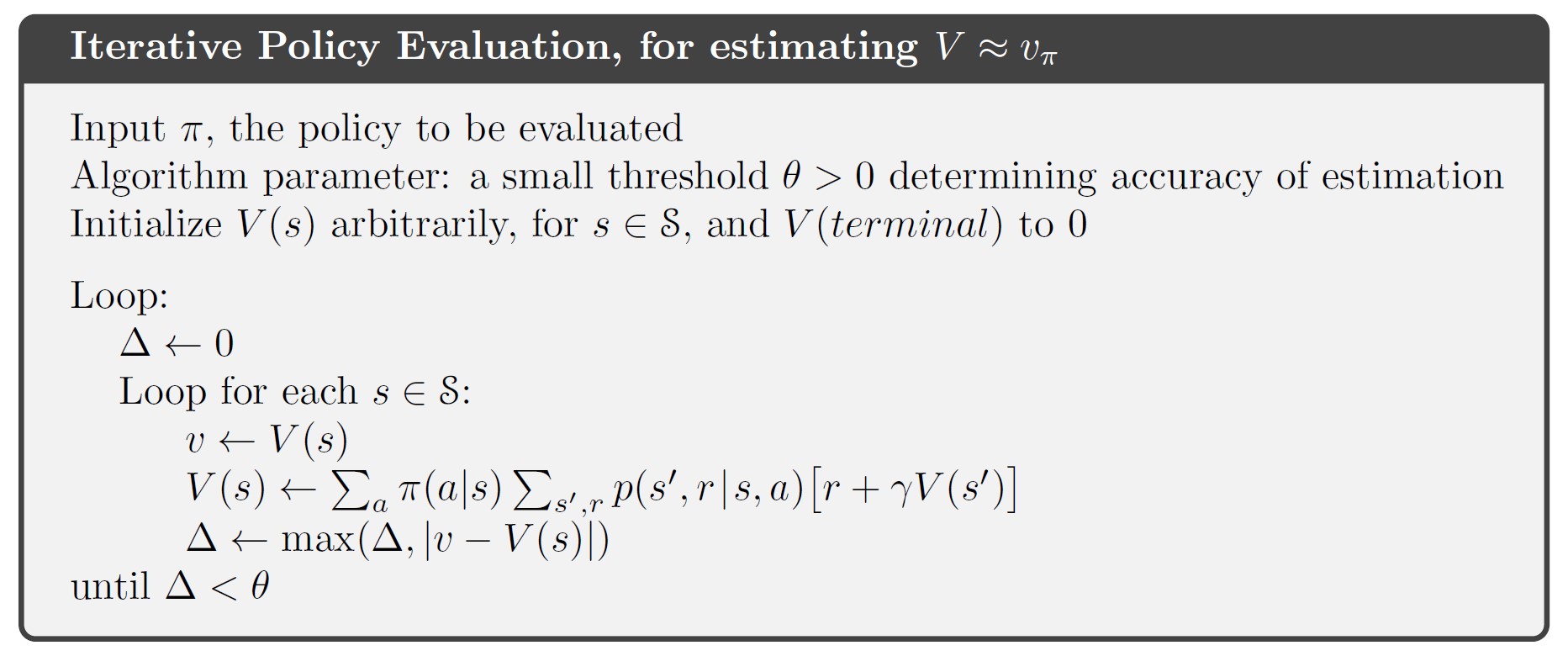 In-place version of iterative policy evaluation
Policy Improvement
Policy Improvement Theorem
Let $\pi$ and $\pi’$ be any pair of deterministic policies such that $\forall s\in\mathcal{S}$,
\[q_\pi(s,\pi'(s))\geq v_\pi(s)\]Then the policy $\pi’$ must be as good as, or better than, $\pi$. That is,
\[v_{\pi'}(s)\geq v_\pi(s),\quad s\in\mathcal{S}\]Special case:
$\pi’$ is identical to $\pi$ except that $\pi’(s)=a\neq \pi(s)$, thus if $q_\pi(s,a)>v_\pi(s)$, then the changed policy $\pi’$ is better than $\pi$.
Extension: consider changes at all states (the new greedy policy $\pi’$)
\[\begin{align} \pi'(s) \dot{=}& {\arg\max_a} q_\pi(s,a)\\ =& {\arg\max_a} \mathbb{E}\big[R_{t+1}+\gamma v_\pi (S_{t+1})\big\vert S_t=s, A_t=a\big]\\ =& {\arg\max_a} \sum_{s',r} p(s',r\vert s,a)\big[r+\gamma v_\pi(s')\big]\\ \end{align}\]When $v_\pi=v_{\pi’}$, the equation turns into Bellman optimality equation. Thus, policy improvement must give us a strictly better policy except when the original policy is already optimal.
Policy Iteration
We can obtain a sequence of monotonically improving policies and value functions:
\[\pi_0 \stackrel{E}{\longrightarrow} v_{\pi_0} \stackrel{I}{\longrightarrow} \pi_1 \stackrel{E}{\longrightarrow} v_{\pi_1} \stackrel{I}{\longrightarrow} \pi_2 \stackrel{E}{\longrightarrow} \cdots \stackrel{I}{\longrightarrow} \pi_\ast \stackrel{E}{\longrightarrow} v_\ast\]where $\stackrel{E}{\longrightarrow}$ policy evaluation, $\stackrel{I}{\longrightarrow}$ policy improvement
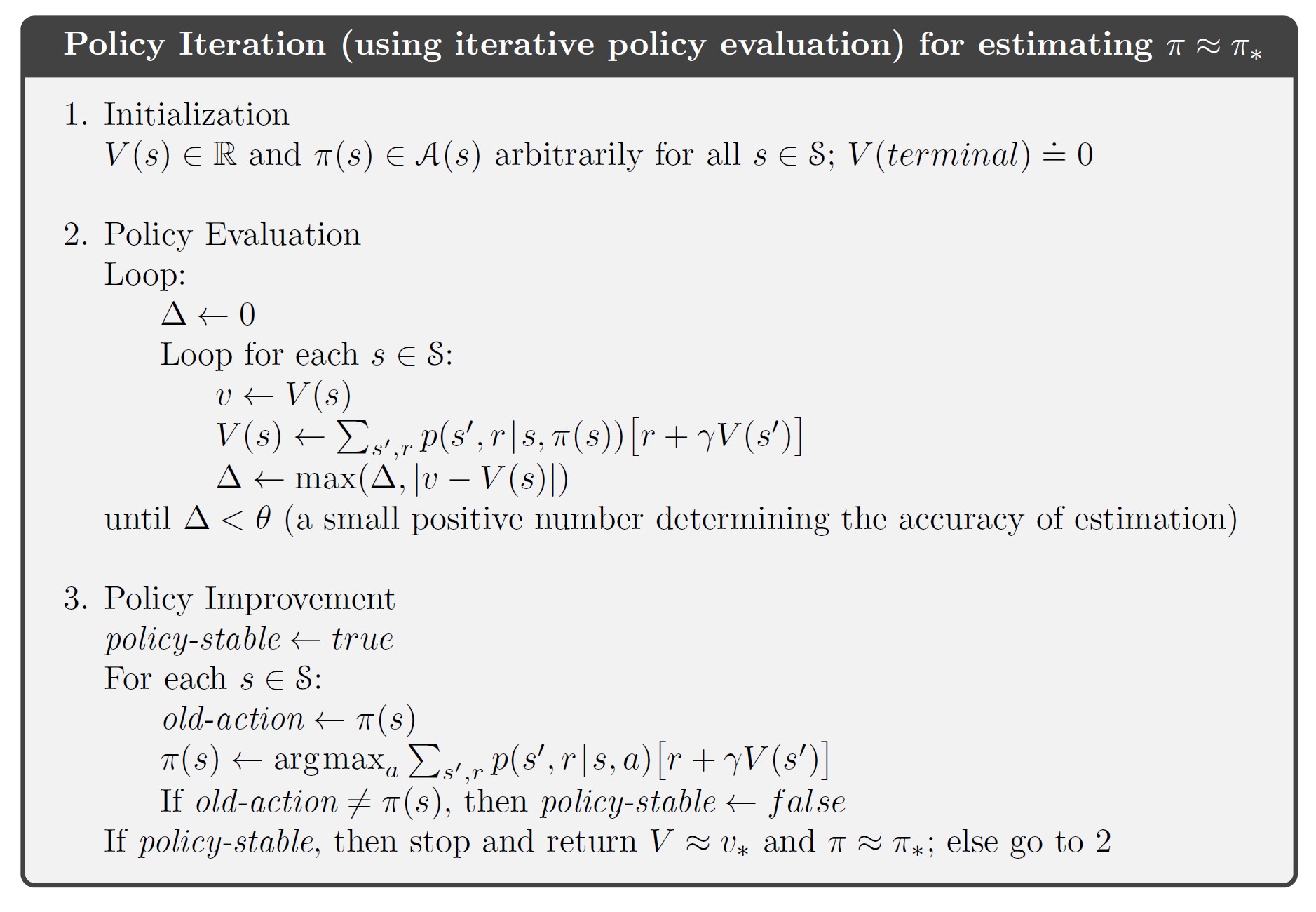 A complete algorithm of policy iteration
Value Iteration
The policy evaluation step of policy iteration can be truncated without losing the convergence guarantees of policy iteration.
An important special case: Value Iteration
Policy evaluation is stopped after one sweep (one update of each state)
\[\begin{align} v_{k+1}(s) \dot{=}& \max_a \mathbb{E}\left[R_{t+1}+\gamma v_k(S_{t+1})\vert S_t=s,A_t=a\right]\\ =&\max_a \sum_{s',r} p(s',r\vert s,a)\big[r+\gamma v_k(s')\big],\quad \forall s\in\mathcal{S} \end{align}\]Another way of understanding:
- Value iteration is obtained simply by turning the Bellman optimality equation into an update rule
- Value iteration update is identical to the policy evaluation update except that it requires the maximum to be taken over all actions
In practice, value iteration terminates once the value function changes by only a small amount in a sweep.
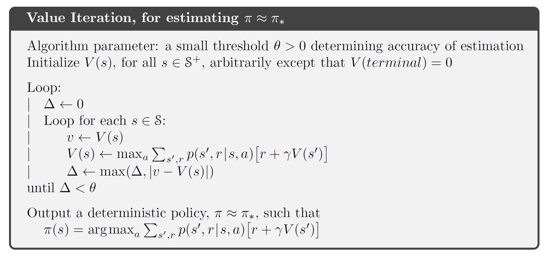 A complete algorithm of value iteration
Asynchronous Dynamic Programming
Asynchronous DP algorithms are in-place iterative DP algorithms that are not organized in terms of systematic sweeps of the state set. These algorithms update the values of states in any order, using whatever values of other states happen to be available. The values of some states may be updated several times before the values of others are updated once. To converge correctly, however, an asynchronous algorithm must continue to update the values of all the states: it can’t ignore any state after some point in the computation. Asynchronous DP algorithms allow great flexibility in selecting states to update.
Avoiding sweeps does not necessarily mean less computation. It just means that an algorithm does not need to be locked into any hopelessly long sweep before it can make progress improving a policy.
Generalized Policy Iteration
Policy iteration consists two simultaneous, interacting processes:
- make the value function consistent with the current policy (policy evaluation)
- make the policy greedy w.r.t. current value function (policy improvement)
Generalized Policy Iteration (GPI): general idea of letting policy-evaluation and policy-improvement processes interact
Almost all RL methods are well described as GPI (all have identifiable policies and value functions, with the policy always being improved w.r.t. value function and the value function always being driven toward the value function for the policy)
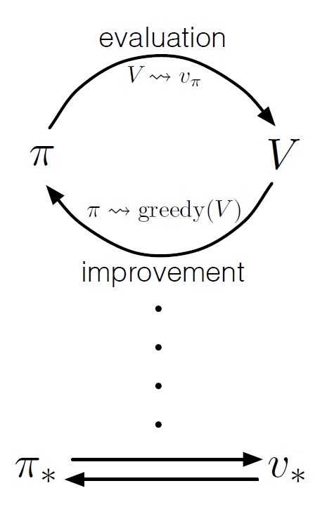
Evaluation and Improvement processes can be viewed as competing and cooperating:
- Making the policy greedy w.r.t. the value function typically makes the value function incorrect for the changed policy
- Making the value function consistent with the policy typically causes that policy no longer to be greedy
- In the long run, find a single joint solution: optimal value function and optimal policy
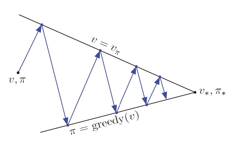 Interaction between evaluation and improvement processes in GPI
Efficiency of Dynamic Programming
- A DP method is guaranteed to find an optimal policy in polynomial time.
- In practice, DP methods can be used with today’s computers to solve MDPs with millions of states.
- On problems with large state spaces, asynchronous DP methods are often preferred.
Summary
Basic Ideas and Algorithms
- Policy evaluation: iterative computation of the value function for a given policy
- Policy improvement: computation of an improved policy given the value function for that policy
- Policy Evaluation + Policy Improvement $\rightarrow$ Policy Iteration & Value Iteration (two most popular DP methods)
- In policy iteration, policy evaluation and policy improvement alternate, each completing before the other begins
- In value iteration, only a single iteration of policy evaluation is performed in between each policy improvement
- Classical DP methods operate in sweeps through the state set, performing an expected update operation on each state. Expected updates are closely related to Bellman equations.
- Not necessary to perform DP methods in complete sweeps through the state set: Asynchronous DP methods
- GPI is the general idea of two interacting processes revolving around an approximate policy and an approximate value function.
- Bootstrapping: all DP methods update estimates on the basis of other estimates (estimates of the values of successor states)
Comments powered by Disqus.