Monte Carlo Methods

MC methods are ways of solving RL problem based on averaging sample returns.
MC methods sample and average returns for each state-action pair and average rewards for each action.
MC methods require only experience - sample sequences of states, actions and rewards from actual or simulated interaction with an environment.

Monte Carlo Prediction

Consider MC methods for learning the state-value function for a given policy

Suppose: estimate the value of a state $s$ under policy $\pi$, $v_\pi(s)$

Each occurrence of state $s$ in an episode is called a visit to $s$ ($s$ may be visited multiple times in the same episode)

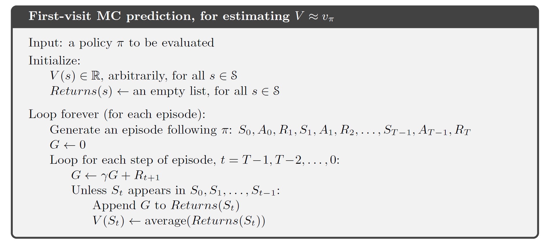
First-visit MC method estimates $v_\pi(s)$ as the average of returns following first visits to $s$ (most widely studied)
Every-visit MC method averages the returns following all visits to $s$

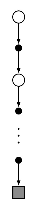
Generalize the idea of backup diagrams to MC algorithms:

For MC estimation of $v_\pi$, the root is a state node, and below it is the entire trajectory of transitions along a particular single episode, ending at the terminal state
MC vs DP
- DP shows all possible transitions, MC shows only those sampled on the one episode
- DP includes only one-step transitions, MC goes all the way to the end of the episode
- DP bootstraps, MC does not (the estimates for each state are independent)

Monte Carlo Estimation of Action Values

If a model is not available, it’s particularly useful to estimate action values rather than state values. Without a model, state values alone are not sufficient to determine a policy.

Policy evaluation problem for action values: estimate $q_\pi(s,a)$, the expected return when starting in state $s$, taking action $a$, and thereafter following policy $\pi$

Visit to a state-action pair: the state $s$ is visited and action $a$ is taken in an episode

Problem: maintaining exploration

If $\pi$ is a deterministic policy, following $\pi$ will observe returns only for one of the actions from each state. Many state-action pairs may never be visited
Solution: every state-action pair has a nonzero probability of being selected as the start (exploring starts)

Exploring starts cannot be relied upon in general, particularly when learning directly from actual interaction with an environment (the starting conditions are unlikely to be so helpful)

Alternative solution: consider only policies that are stochastic with a nonzero probability of selecting actions in each state

Monte Carlo Control

Consider using MC estimation in control (approximate optimal policies)

Idea of GPI: maintain both an approximate policy and an approximate value function

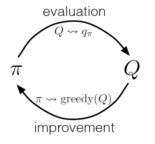
Consider a MC version of classical policy iteration: perform alternating complete steps of policy evaluation and policy improvement, beginning with an arbitrary policy $\pi_0$ and ending with the optimal policy and optimal action-value function:

\[\pi_0 \stackrel{E}{\longrightarrow} q_{\pi_0} \stackrel{I}{\longrightarrow} \pi_1 \stackrel{E}{\longrightarrow} q_{\pi_1} \stackrel{I}{\longrightarrow} \pi_2 \stackrel{E}{\longrightarrow} \cdots \stackrel{I}{\longrightarrow} \pi_\ast \stackrel{E}{\longrightarrow} q_\ast\]

Policy improvement: construct each $\pi_{k+1}$ as the greedy policy w.r.t. $q_{\pi_k}$

\[\pi(s)\dot{=} \arg\max_a q(s,a)\]

The policy improvement theorem applies to $\pi_k$ and $\pi_{k+1}$
Proof:
\[\begin{align} q_{\pi_k}(s,\pi_{k+1}(s))\dot{=}& q_{\pi_k}(s, \arg\max_a q_{\pi_k}(s,a))\\ =& \max_a q_{\pi_k}(s,a)\\ \geq& q_{\pi_k}(s,\pi_k(s))\\ \geq& v_{\pi_k}(s)\quad \forall s\in\mathcal{S}\\ \end{align}\]

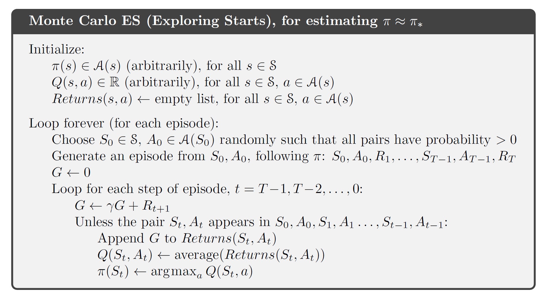
Two unlikely assumptions:

The episodes have exploring starts
Policy evaluation could be done with an infinite number of episodes

Now remove the second assumption

Solution 1: idea of approximating $q_{\pi_k}$
Make measurements and assumptions to obtain bounds on the magnitude and probability of error in the estimates, and then take sufficient steps to assure these bounds are sufficiently small
Solution 2: give up complete policy evaluation before returning to policy improvement
On each evaluation step, move the value function toward $q_{\pi_k}$

Monte Carlo Control without Exploring Starts

On-policy methods attempt to evaluate or improve the policy that is used to make decisions
Off-policy methods attempt to evaluate or improve the policy different from that used to generate the data

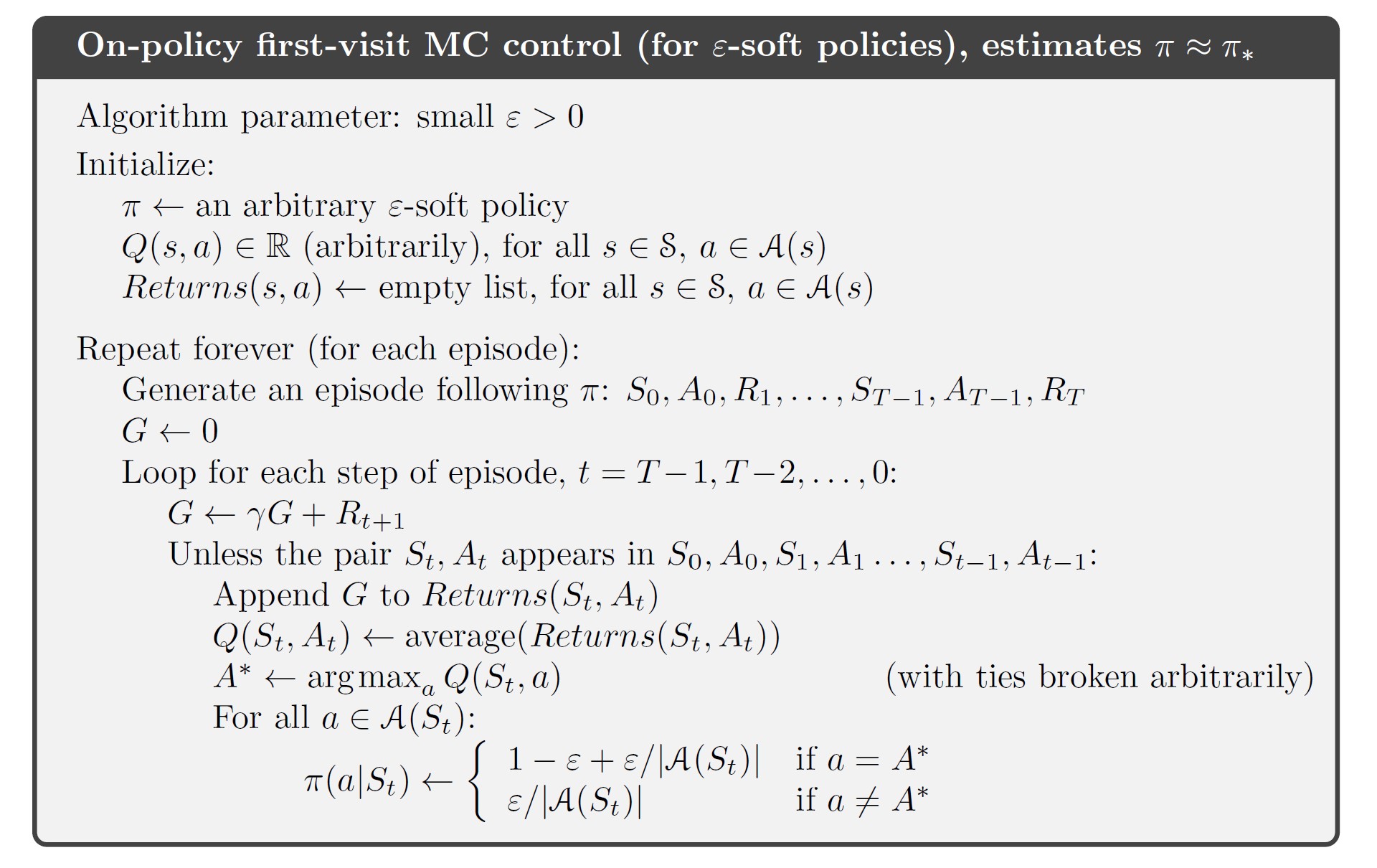
On-policy Methods without Exploring Starts

Soft policy: $\pi(a\vert s)>0,~\forall s\in\mathcal{S},a\in\mathcal{A}(s)$, but gradually shifted closer to a deterministic optimal policy
$\varepsilon$-soft policies: $\pi(a\vert s)\geq \frac{\varepsilon}{\vert\mathcal{A}(s)\vert}$ for all states and actions
$\varepsilon$-greedy policies: most of the time choose an action that has maximal estimated action value, but with probability $\varepsilon$ select an action at random
- Probability of selecting nongreedy actions: $\frac{\varepsilon}{\vert \mathcal{A}(s)\vert}$
- Probability of selecting greedy actions: $1-\varepsilon+\frac{\varepsilon}{\vert \mathcal{A}(s)\vert}$

In on-policy MC method, move the policy only to an $\varepsilon$-greedy policy. For any $\varepsilon$-soft policy $\pi$, any $\varepsilon$-greedy policy w.r.t. $q_\pi$ is better than or equal to $\pi$

Let $\pi’$ be the $\varepsilon$-greedy policy, prove that $\pi’\geq\pi$
\[\begin{align} q_\pi(s,\pi'(s)) &= \sum_a \pi'(a\vert s) q_\pi(s,a)\\ &= \frac{\varepsilon}{\vert \mathcal{A}(s)\vert}\sum_a q_\pi(s,a) + (1-\varepsilon)\max_a q_\pi(s,a)\\ &\geq \frac{\varepsilon}{\vert \mathcal{A}(s)\vert}\sum_a q_\pi(s,a) + (1-\varepsilon)\sum_a\frac{\pi(a\vert s)-\frac{\varepsilon}{\vert \mathcal{A}(s)\vert}}{1-\varepsilon}q_\pi(s,a)\\ &= \frac{\varepsilon}{\vert \mathcal{A}(s)\vert}\sum_a q_\pi(s,a) - \frac{\varepsilon}{\vert \mathcal{A}(s)\vert}\sum_a q_\pi(s,a) + \sum_a \pi(a\vert s)q_\pi(s,a)\\ &= v_\pi(s) \end{align}\]

The cost of eliminating the assumption of exploring starts is that we only achieve the best policy among the $\varepsilon$-soft policies.

All learning control methods face a dilemma: They seek to learn action values conditional on subsequent optimal behavior, but they need to behave non-optimally in order to explore all actions (to find the optimal actions). The on-policy approach is a compromise – it learns action values not for the optimal policy, but for a near-optimal policy that still explores. A more straightforward approach is to use two policies (off-policy approach)

Off-policy Prediction via Importance Sampling

Target policy: policy being learned about
Behavior policy: policy used to generate behavior
On-policy vs Off-policy
- On-policy methods are generally simpler and are consider first.
- Off-policy methods require additional concepts and notation, and are often of greater variance and are slower to converge because the data is due to a different policy. But off-policy methods are more powerful and general.

Consider the prediction problem (both target and behavior policies are fixed):

We wish to estimate $v_\pi$ or $q_\pi$, but all we have are episodes following another policy $b\neq\pi$ ($\pi$ is the target policy, $b$ is the behavior policy)

Assumption of coverage:

In order to use episodes from $b$ to estimate values for $\pi$, it’s required that every action taken under $\pi$ is also taken, at least occasionally, under $b$.

\[\pi(a\vert s)>0 \Rightarrow b(a\vert s)>0\]

Almost all off-policy methods utilize importance sampling, a general technique for estimating expected values under on distribution given samples from another.

Apply importance sampling to off-policy learning: weight returns according to the relative probability of their trajectories occurring under the target and behavior policies, called the importance-sampling ratio.

Given a starting state $S_t$, the probability of the subsequent state-action trajectory $A_t, S_{t+1}, A_{t+1},\dots, S_T$, occurring under any policy $\pi$ is

\[\begin{align} P &\{A_t, S_{t+1}, A_{t+1},\dots, S_T\vert S_t,A_{t:T-1}\sim\pi \}\\ &= \pi(A_t\vert S_t)p(S_{t+1}\vert S_t,A_t)\pi(A_{t+1}\vert S_{t+1})\cdots p(S_T\vert S_{T-1}, A_{T-1})\\ &= \prod_{k=t}^{T-1} \pi(A_k\vert S_k) p(S_{k+1}\vert S_k,A_k)\\ \end{align}\]

where $p$ is the state-transition probability function defined [before][https://oscarjin.github.io/posts/rl-notes-3/#the-agent-environment-interface]

The relative probability of the trajectory under the target and behavior policies (the importance-sampling ratio):

\[\rho_{t:T-1} \dot{=} \frac{\prod_{k=t}^{T-1} \pi(A_k\vert S_k) p(S_{k+1}\vert S_k,A_k)}{\prod_{k=t}^{T-1} b(A_k\vert S_k) p(S_{k+1}\vert S_k,A_k)}=\prod_{k=t}^{T-1} \frac{\pi(A_k\vert S_k) }{b(A_k\vert S_k)}\]

Although the trajectory probabilities depend on the MDP’s transition probabilities, which are generally unknown, the importance-sampling ratio depends only on the two policies and the sequence, not on MDP.

The ratio $\rho_{t:T-1}$ transforms the returns to have the right expected value:

\[\mathbb{E}[\rho_{t:T-1}G_t\vert S_t=s]=v_\pi(s)\]

Now give a MC algorithm that averages returns from a batch of observed episodes following policy $b$ to estimate $v_\pi(s)$

Here number the time steps that increase across episode boundaries to refer to particular steps in particular episodes
$\mathcal{J}(s)$ – the set of all time steps in which state $s$ is visited (for a first-visit method, only include time steps that are first visits to $s$ within their episodes)
$T(t)$ – the first time of termination following time $t$
$G_t$ – the return after $t$ up through $T(t)$
${G_t}_{t\in\mathcal{J}(s)}$ – returns that pertain to state $s$
${\rho_{t:T(t)-1}}_{t\in\mathcal{J}(s)}$ – corresponding importance-sampling ratios

To estimate $v_\pi(s)$, simply scale the returns by the ratios and average the results:

Ordinary importance sampling

\[V(s) \dot{=} \frac{\sum_{t\in\mathcal{J}(s)}\rho_{t:T(t)-1}G_t}{\vert \mathcal{J}(s)\vert}\]

Weighted importance sampling

\[V(s) \dot{=} \frac{\sum_{t\in\mathcal{J}(s)}\rho_{t:T(t)-1}G_t}{\sum_{t\in\mathcal{J}(s)}\rho_{t:T(t)-1}}\]

Difference between the first-visit methods of the two kinds of importance sampling (biases and variances)
- Ordinary importance sampling is unbiased; weighted importance sampling is biased
- Variance of ordinary importance sampling is in general unbounded because the variance of the ratios can be unbounded; in the weighted importance sampling, the largest weight on any single return is one
- In practice, the weighted estimator is usually has lower variance and is strongly preferred.
The every-visit methods for ordinary and weighted importance sampling are both biased. The bias falls asymptotically to zero as the number of samples increases. In practice, every-visit methods are often preferred because they remove the need to keep track of which states have been visited and because they are much easier to extend to approximations.

Incremental Implementation (for Off-policy Methods)

In MC methods we average returns.

Ordinary Importance Sampling

Returns are scaled by the importance sampling ratio $\rho_{t:T(t)-1}$, then simply averaged.

Weighted Importance Sampling

Suppose a sequence of returns $G_1,G_2,\dots,G_{n-1}$, all starting in the same state and each with a corresponding random weight $W_i$ (eg. $W_i=\rho_{t_i:T(t_i)-1}$)

Form the estimate:

\[V_n\dot{=}\frac{\sum_{k=1}^{n-1} W_kG_k}{\sum_{k=1}^{n-1}W_k},\quad n\geq 2\]

Introduce $C_{n+1}\dot{=} C_n+W_{n+1}$ where $C_0\dot{=}0$

Update rule for $V_n$

\[V_{n+1}=\dot{=} V_n+\frac{W_n}{C_n}\big[G_n-V_n\big],\quad n\geq 1\]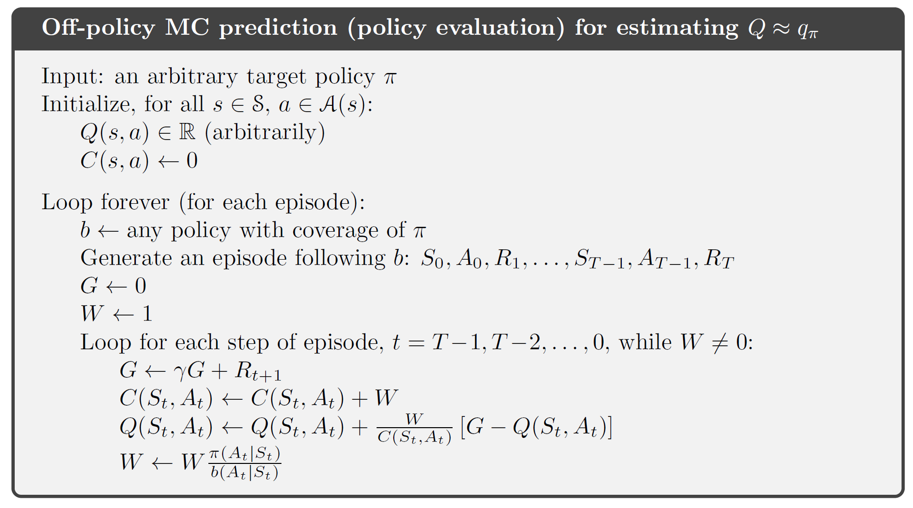

A complete episode-by-episode incremental algorithm for MC policy evaluation (for the off-policy case, using weighted importance sampling)

Off-policy Monte Carlo Control

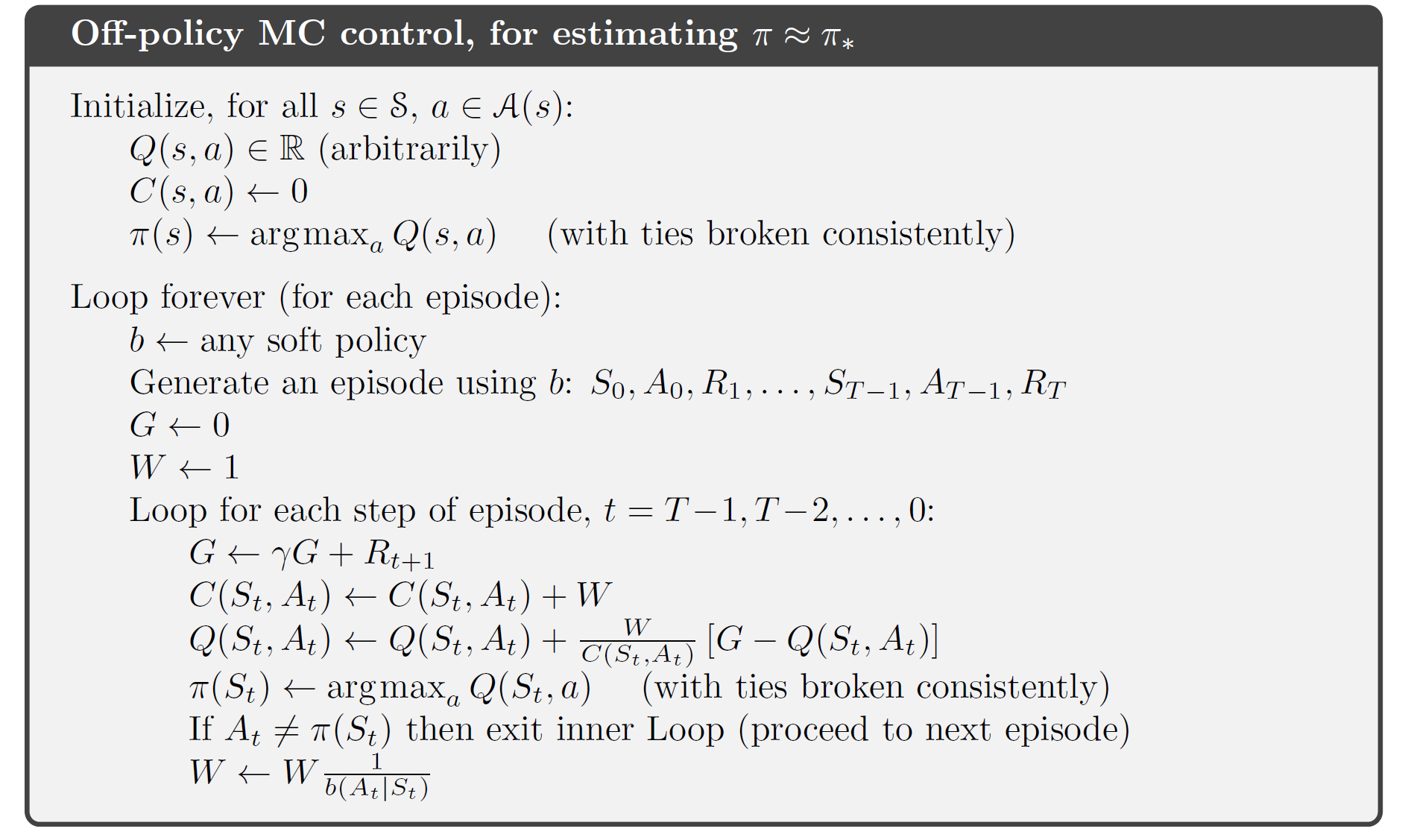An off-policy MC control method based on GPI and weighted importance sampling

The target policy $\pi\approx\pi_\ast$ is the greedy policy w.r.t. $Q$ (estimate of $q_\ast$). The behavior policy $b$ is random but $\varepsilon$-soft to assure convergence of $\pi$ to the optimal policy.

Summary

MC methods learn value functions and optimal policies from experience in the form of sample episodes.

Advantages over DP methods:

They can be used to learn optimal behavior directly from interaction with the environment, with no model of the environment’s dynamics.
They can be used with simulation or sample models. For many applications it is easy to simulate sample episodes even though it is difficult to construct the kind of explicit model of transition probabilities required by DP methods.
It is easy and efficient to focus Monte Carlo methods on a small subset of the states.
They may be less harmed by violations of the Markov property. This is because they do not update their value estimates on the basis of the value estimates of successor states (or they do not bootstrap).

MC methods follow the overall schema of GPI involving interacting processes of policy evaluation and policy improvement.

In policy evaluation process, they simply average many returns that start in the state.
In control methods, they approximate action-value functions, because these can be used to improve the policy without requiring a model of the environment’s transition dynamics.
MC methods intermix policy evaluation and policy improvement steps on an episode-by-episode basis, and can be incrementally implemented on an episode-by-episode basis.

Maintaining sufficient exploration:

Exploring starts are unlikely in learning from real experience, so we introduce off-policy methods (learning the value function of a target policy from data generated by a different behavior policy).
Off-policy methods are based on importance sampling, that is, weighting returns by the ratio of the probabilities of taking the observed actions under the two policies,