
TD learning is a combination of MC ideas and DP ideas.
- Like MC methods, TD methods can learn directly from raw experience without a model of the environments dynamics.
- Like DP, TD methods update estimates based in part on other learned estimates, without waiting for a final outcome.
- For the control problem (finding an optimal policy), DP, TD and MC all use some variation of GPI.
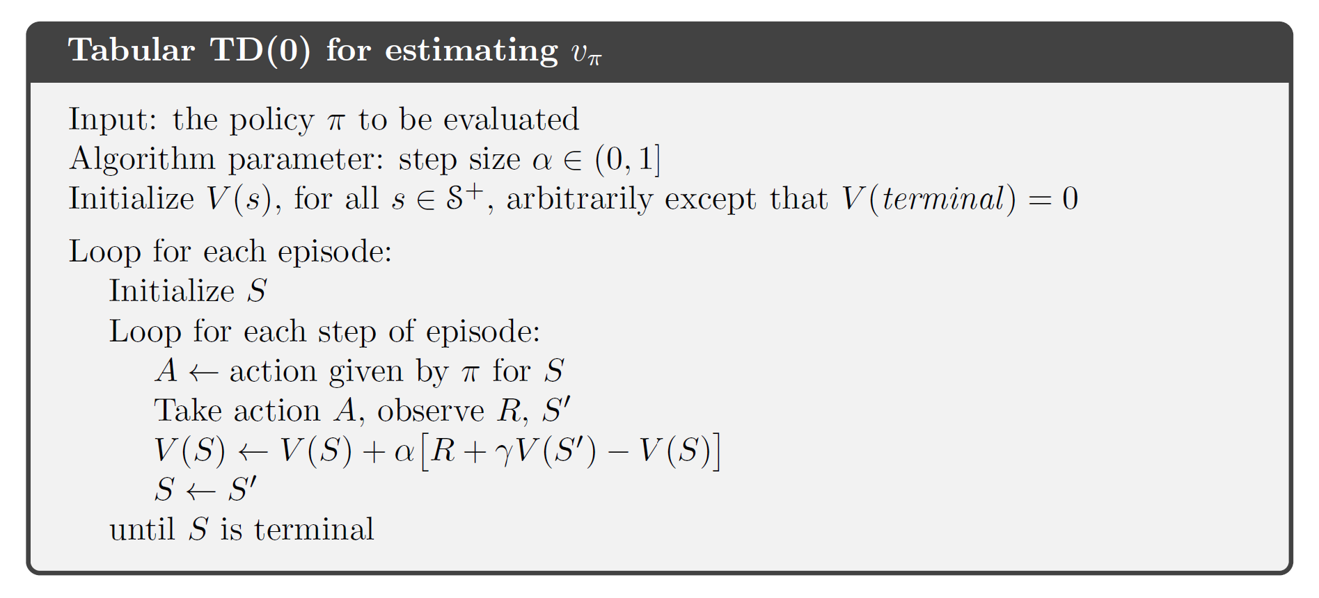
TD Prediction
Both TD and MC methods use experience to solve the prediction problem.
MC methods wait until the return following the visit is known, then use that return as a target for $V(S_t)$
\[V(S_t) \leftarrow V(S_t)+\alpha \big[G_t-V(S_t)\big]\]MC methods must wait until the end of the episode to determine the increment to $V(S_t)$ (only then is $G_t$ known), TD methods need to wait only until the next time step. At time $t+1$ they immediately form a target and make a useful update using the observed reward $R_{t+1}$ and the estimate $V(S_{t+1})$
\[V(S_t)\leftarrow V(S_t)+\alpha\big[R_{t+1}+\gamma V(S_{t+1})-V(S_t)\big]\]The target for MC update is $G_t$, whereas the target for the TD update is $R_{t+1}+\gamma V(S_{t+1})$.
This TD method is called TD(0) or one-step TD.
TD(0) is a bootstrapping method (it bases its update in part on an existing estimate). TD methods combine the sampling of MC with the bootstrapping of DP.
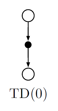 Backup diagram for tabular TD(0)
The value estimate for the state node at the top of the backup diagram is updated on the basis of the one sample transition from it to the immediately following state. We refer to TD updates as sample updates because they involve looking ahead to a sample successor state (or state–action pair), using the value of the successor and the reward along the way to compute a backed-up value, and then updating the value of the original state (or state–action pair) accordingly.
TD error: difference between the estimated value of $S_t$ and the better estimate $R_{t+1}+\gamma V(S_{t+1})$
\[\delta_t\dot{=} R_{t+1}+\gamma V(S_{t+1})-V(S_t)\]If the array $V$ doesn’t change during the episode, then the MC error can be written as a sum of TD errors:
\[\begin{align} G_t-V(S_t) &= R_{t+1}+\gamma G_{t+1}-V(S_t)+\gamma V(S_{t+1})-\gamma V(S_{t+1})\\ &= \delta_t+\gamma (G_{t+1}-V(S_{t+1}))\\ &= \delta_t+\gamma\delta_{t+1}+\gamma^2(G_{t+2}-V(S_{t+2}))\\ &= \cdots\\ &=\sum_{k=t}^{T-1}\gamma^{k-t}\delta_k \end{align}\]If the step size is small, it may still hold approximately.
Advantages of TD Prediction Methods
TD methods update their estimates based in part on other estimates (they bootstrap),
- TD methods don’t require a model of the environment, of its reward and next-state probability distributions. (advantage over DP)
- TD methods are naturally implemented in an online, fully incremental fashion. (advantage over MC, with MC methods one must wait until the end of an episode)
- For any fixed policy $\pi$, TD(0) has been proved to converge to $v_\pi$, in the mean for a constant step-size parameter if it’s sufficiently small, and with probability 1 if the step-size parameter decreases according to the usual stochastic approximation conditions. TD methods have usually been found to converge faster than constant-$\alpha$ MC methods on stochastic tasks.
Optimality of TD(0)
Batch updating: Given an approximate value function, $V$ , the increments are computed for every time step $t$ at which a nonterminal state is visited, but the value function is changed only once, by the sum of all the increments. Then all the available experience is processed again with the new value function to produce a new overall increment, and so on, until the value function converges.
As long as $\alpha$ is sufficiently small, TD(0) and constant-$\alpha$ MC both converge, but to two different answers.
Batch MC methods always find the estimates that minimize MSE on the training set, whereas batch TD(0) always find the estimates that would be exactly correct for the maximum-likelihood model of the Markov process.
In general, TD(0) converges to the certainty-equivalence estimate (equivalent to assuming that the estimate of the underlying process was known with certainty rather than being approximated).
Sarsa: On-policy TD Control
The use of TD prediction methods for the control problem
Two classes: on-policy & off-policy
- Learn an action-value function
If $S_{t+1}$ is terminal, then $Q(S_{t+1},A_{t+1}) \dot{=} 0$
This rule uses every element of the quintuple of events, $(S_t, A_t, R_{t+1}, S_{t+1},A_{t+1})$, that make up a transition from one state-action pair to the next (this quintuple give rise to the name Sarsa)
- Design an on-policy control algorithm based on the Sarsa prediction method
As in all on-policy methods, continually estimate $q_\pi$ for the behavior policy $\pi$ and at the same time change $\pi$ toward greediness w.r.t. $q_\pi$.
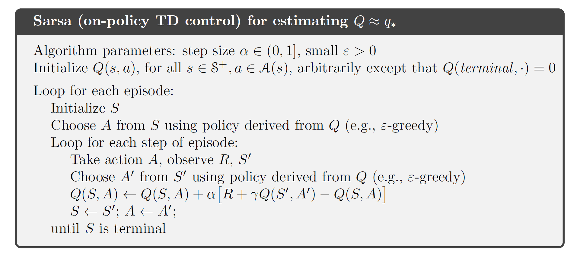 General form of the Sarsa control algorithm
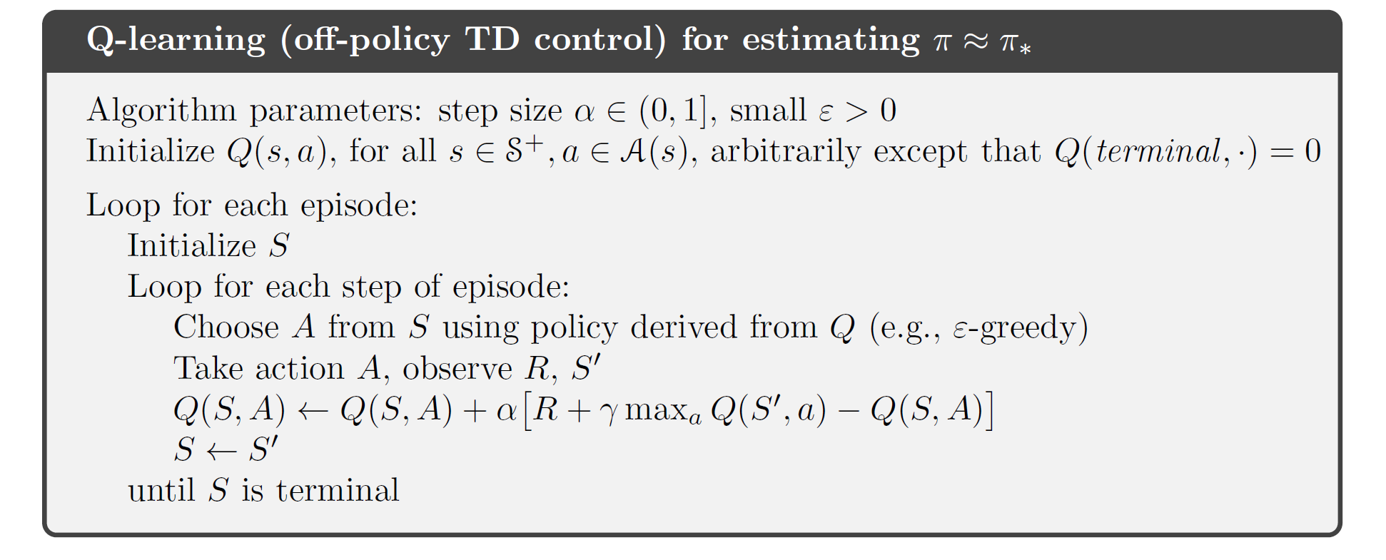
Q-learning: Off-policy TD Control
Update rule:
\[Q(S_t,A_t) \leftarrow Q(S_t,A_t) +\alpha\big[R_{t+1} +\gamma\max_aQ(S_{t+1},a) - Q(S_t,A_t) \big]\]The learned action-value function, $Q$, directly approximates the optimal action-value function, $q_\ast$, independent of the policy being followed.
Expected Sarsa
Consider the learning algorithm that is just like Q-learning except that instead of the maximum over next state-action pairs it uses the expected value, taking into account how likely each action is under the current policy.
Update rule:
\[\begin{align} Q(S_t,A_t)&\leftarrow Q(S_t,A_t)+\alpha \big[R_{t+1} + \gamma\mathbb{E}_\pi[Q(S_{t+1},A_{t+1})\vert S_{t+1}] - Q(S_t,A_t) \big]\\ &= Q(S_t,A_t)+\alpha \big[R_{t+1} + \gamma\sum_a \pi(a\vert S_{t+1})Q(S_{t+1},a)-Q(S_t,A_t) \big]\\ \end{align}\]Given the next state $S_{t+1}$, this algorithm moves deterministically in the same direction as Sarsa moves in expectation, and accordingly it’s called Expected Sarsa.
Expected Sarsa performs slightly better than Sarsa, but is more complex computationally than Sarsa.
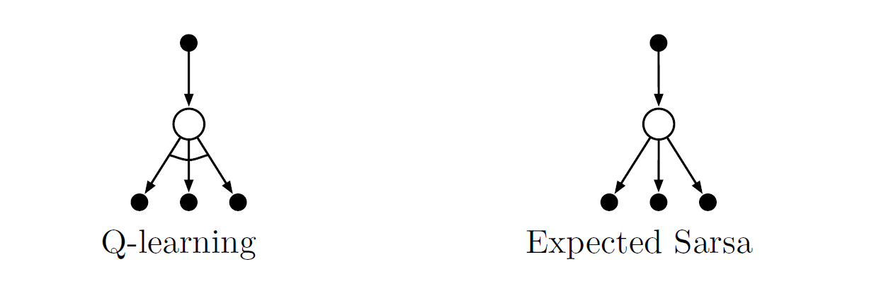 The backup diagrams for Q-learning and Expected Sarsa
Maximization Bias and Double Learning
All the control algorithms discussed so far involve maximization in the construction of their target policies. In these algorithms, a maximum over estimated values is used implicitly as an estimate of the maximum value, which can lead to a significant positive bias, called maximization bias.
Understand maximization bias:
Consider a single state $s$ where there are many actions $a$ whose true values $q(s,a)$ are all zero but whose estimated values $Q(s,a)$ are uncertain and thus distributed some above and some below zero. The maximum of the true values is zero, but the maximum of the estimates is positive.
Avoid maximization bias: the idea of double learning
Use one estimate $Q_1(a)$ to determine the maximizing action $A^\ast=\arg\max_a Q_1(a)$, and the other $Q_2(a)$ to provide the estimate of its value $Q_2(A^\ast)=Q_2(\arg\max_aQ_1(a))$
This estimate will then be unbiased: $\mathbb{E}[Q_2(A^\ast)]=q(A^\ast)$
Note:
- Although we learn two estimates, only one estimate is updated on each play.
- Double learning doubles the memory requirements, but does not increase the amount of computation per step.
Update rule of Double Q-learning:
\[Q_1(S_t,A_t)\leftarrow Q_1(S_t,A_t)+\alpha \big[R_{t+1} +\gamma Q_2(S_{t+1},\arg\max_a Q_1(S_{t+1},a))-Q_1(S_t,A_t) \big]\]Update $Q_1$ and $Q_2$ each with 0.5 probability.
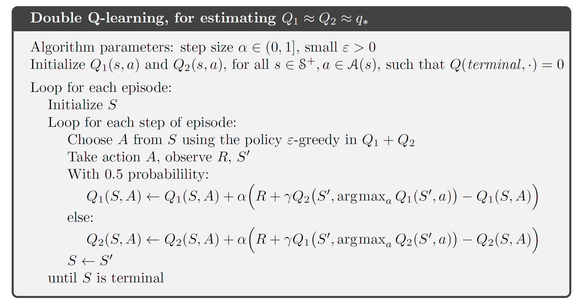 A complete algorithm for Double Q-learning
Comments powered by Disqus.